function main_conservative_pendulum_simulation()
phys.m = 2.0;
phys.L = 1.2;
phys.g = 9.81;
phys.d = phys.L / 2;
phys.I_O = (1/3) * phys.m * phys.L^2;
omega0 = sqrt(phys.m * phys.g * phys.d / phys.I_O);
T0 = 2 * pi / omega0;
t_span = [0, 10];
theta0_list = [0.1, 0.2, 0.3, 0.5, 0.8, 1.0, 1.5, 2.0, 2.5, 3.0];
options_normal = odeset('RelTol', 1e-11, 'AbsTol', 1e-13);
options_events = odeset('RelTol', 1e-11, 'AbsTol', 1e-13, 'Events', @zero_crossing_event);
fprintf('\n=====================================================================================\n');
fprintf(' 不同初始释放角下复摆非线性周期与线性周期对比计算报表(软弹簧非线性效应)\n');
fprintf('=====================================================================================\n');
fprintf(' 初始释放角 theta0 (rad)\t初始几何角度(度)\t线性理论周期 T0(s)\tMATLAB数值周期T(s)\t周期相对偏差率\n');
traj_data = cell(length(theta0_list), 1);
for idx = 1:length(theta0_list)
theta0 = theta0_list(idx);
init_cond = [theta0; 0.0];
sol = ode45(@(t,x) odefcn_nonlinear(t,x,phys), t_span, init_cond, options_events);
traj_data{idx} = sol;
if ~isempty(sol.xe)
pos_cross = find(sol.ye(2,:) > 0);
if length(pos_cross) >= 2
T = sol.xe(pos_cross(2)) - sol.xe(pos_cross(1));
else
T = NaN;
end
else
T = NaN;
end
if ~isnan(T)
err = (T - T0)/T0 * 100;
fprintf(' %.1f\t\t\t%.1f\t\t\t%.4f\t\t\t%.4f\t\t\t%.2f%%\n',...
theta0, rad2deg(theta0), T0, T, err);
end
end
fprintf('=====================================================================================\n');
init_small = [0.1; 0.0];
init_medium = [1.5; 0.0];
init_large = [3.0; 0.0];
[tA_lin, xA_lin] = ode45(@(t,x) odefcn_linear(t,x,phys), t_span, init_small, options_normal);
[tA_non, xA_non] = ode45(@(t,x) odefcn_nonlinear(t,x,phys), t_span, init_small, options_normal);
[tB_lin, xB_lin] = ode45(@(t,x) odefcn_linear(t,x,phys), t_span, init_medium, options_normal);
[tB_non, xB_non] = ode45(@(t,x) odefcn_nonlinear(t,x,phys), t_span, init_medium, options_normal);
sol_large_non = ode45(@(t,x) odefcn_nonlinear(t,x,phys), t_span, init_large, options_events);
figure('Color', [1 1 1], 'Position', [100, 100, 1000, 800]);
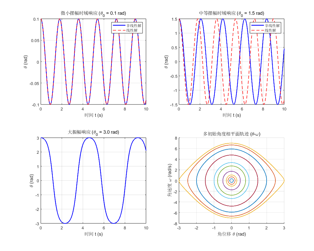
subplot(2, 2, 1);
plot(tA_non, xA_non(:,1), 'b-', 'LineWidth', 1.8); hold on;
plot(tA_lin, xA_lin(:,1), 'r--', 'LineWidth', 1.2);
title('微小摆幅时域响应 (\theta_0 = 0.1 rad)');
xlabel('时间 t (s)'); ylabel('\theta (rad)');
legend('非线性解','线性解','Location','northeast'); grid on;
subplot(2, 2, 2);
plot(tB_non, xB_non(:,1), 'b-', 'LineWidth', 1.8); hold on;
plot(tB_lin, xB_lin(:,1), 'r--', 'LineWidth', 1.2);
title('中等摆幅时域响应 (\theta_0 = 1.5 rad)');
xlabel('时间 t (s)'); ylabel('\theta (rad)');
legend('非线性解','线性解','Location','northeast'); grid on;
subplot(2, 2, 3);
plot(sol_large_non.x, sol_large_non.y(1,:), 'b-', 'LineWidth', 1.8);
title('大振幅响应 (\theta_0 = 3.0 rad)');
xlabel('时间 t (s)'); ylabel('\theta (rad)'); grid on;
subplot(2, 2, 4); hold on; grid on;
colors = lines(length(theta0_list));
for idx = 1:length(theta0_list)
sol = traj_data{idx};
plot(sol.y(1,:), sol.y(2,:), 'Color', colors(idx,:), 'LineWidth', 1.4);
end
title('多初始角度相平面轨迹 (\theta-\omega)');
xlabel('角位移 \theta (rad)');
ylabel('角速度 \omega (rad/s)');
fprintf('\n================== 复摆保守动力学计算报表 ==================\n');
fprintf('刚体物理参量:\n');
fprintf(' - 直杆质量 m = %.2f kg, 长度 L = %.2f m\n', phys.m, phys.L);
fprintf(' - 转动惯量 I_O = %.5f kg·m², 固有频率 w_0 = %.4f rad/s\n', phys.I_O, omega0);
fprintf('周期分析结果:\n');
fprintf(' - 线性理论周期 T_0 = %.5f s\n', T0);
if ~isempty(sol_large_non.xe)
idx_pos = find(sol_large_non.ye(2,:) > 0);
if length(idx_pos) >= 2
T_large = sol_large_non.xe(idx_pos(2)) - sol_large_non.xe(idx_pos(1));
fprintf(' - 大偏幅数值周期 T = %.5f s\n', T_large);
fprintf(' - 非线性延迟率 = %.2f %%\n', (T_large - T0)/T0 * 100);
end
end
verify_hamiltonian_conservation(sol_large_non, phys);
end
function dxdt = odefcn_nonlinear(~, x, phys)
dxdt = [x(2); -(phys.m*phys.g*phys.d/phys.I_O)*sin(x(1))];
end
function dxdt = odefcn_linear(~, x, phys)
dxdt = [x(2); -(phys.m*phys.g*phys.d/phys.I_O)*x(1)];
end
function [value, isterminal, direction] = zero_crossing_event(~, x)
value = x(1);
isterminal = 0;
direction = 0;
end
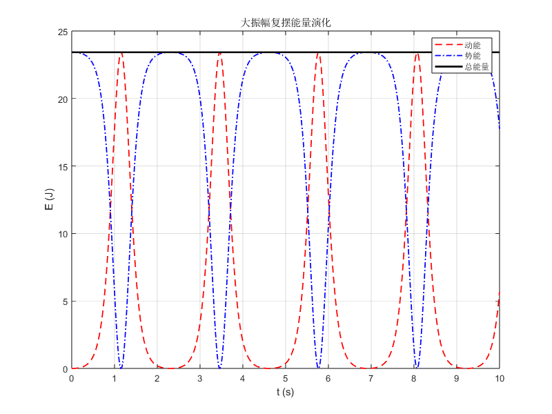
function verify_hamiltonian_conservation(sol, phys)
theta = sol.y(1,:);
omega = sol.y(2,:);
E_kin = 0.5 * phys.I_O * omega.^2;
E_pot = phys.m * phys.g * phys.d * (1 - cos(theta));
E_total = E_kin + E_pot;
figure('Color','w','Position',[200,200,800,600]);
plot(sol.x, E_kin, 'r--','LineWidth',1.3); hold on;
plot(sol.x, E_pot, 'b-.','LineWidth',1.3);
plot(sol.x, E_total, 'k-','LineWidth',2.0);
title('大振幅复摆能量演化');
xlabel('t (s)'); ylabel('E (J)');
legend('动能','势能','总能量'); grid on;
max_drift = max(abs(E_total - E_total(1))) / E_total(1) * 100;
fprintf('\n哈密顿守恒校对:\n');
fprintf(' - 初始能量 H0 = %.6f J\n', E_total(1));
fprintf(' - 最大能量漂移 = %.5e %% \n', max_drift);
end
=====================================================================================
           不同初始释放角下复摆非线性周期与线性周期对比计算报表(软弹簧非线性效应)
=====================================================================================
  初始释放角 theta0 (rad)	初始几何角度(度)	线性理论周期 T0(s)	MATLAB数值周期T(s)	周期相对偏差率
          0.1			5.7			1.7943			1.7954			0.06%
          0.2			11.5			1.7943			1.7988			0.25%
          0.3			17.2			1.7943			1.8044			0.57%
          0.5			28.6			1.7943			1.8227			1.59%
          0.8			45.8			1.7943			1.8688			4.15%
          1.0			57.3			1.7943			1.9133			6.63%
          1.5			85.9			1.7943			2.0849			16.20%
          2.0			114.6			1.7943			2.3844			32.89%
          2.5			143.2			1.7943			2.9480			64.30%
          3.0			171.9			1.7943			4.6135			157.12%
=====================================================================================

================== 复摆保守动力学计算报表 ==================
刚体物理参量:
  - 直杆质量 m = 2.00 kg, 长度 L = 1.20 m
  - 转动惯量 I_O = 0.96000 kg·m², 固有频率 w_0 = 3.5018 rad/s
周期分析结果:
  - 线性理论周期 T_0 = 1.79428 s
  - 大偏幅数值周期 T = 4.61352 s
  - 非线性延迟率 = 157.12 %

哈密顿守恒校对:
  - 初始能量 H0 = 23.426192 J
  - 最大能量漂移 = 6.56775e-10 %